What Factors do Influence the Nominal Risk-Free Rate (NRFR)?

An investor would be willing to forgo current consumption in order to increase future consumption at a rate of exchange called the risk-free rate of interest. This rate of exchange was measured in real terms because we assume that investors want to increase the consumption of actual goods and services rather than consuming the same amount that had come to cost more money. Therefore, when we discuss rates of interest, we need to differentiate between real rates of interest that adjust for changes in the general price level, as opposed to nominal rates of interest that are stated in money terms. That is, nominal rates of interest that prevail in the market are determined by real rates of interest, plus factors that will affect the nominal rate of interest, such as the expected rate of inflation and the monetary environment. It is important to understand these factors.

Notably, the variables that determine the RRFR change only gradually because we are concerned with long-run real growth. Therefore, you might expect the required rate on a risk-free investment to be quite stable over time. As discussed in connection with Exhibit 1.5, rates on three-month T-bills were not stable over the period from 2004 to 2010. This is demonstrated with additional observations in Exhibit 1.6, which contains yields on T-bills for the period 1987–2010.

Investors view T-bills as a prime example of a default-free investment because the government has unlimited ability to derive income from taxes or to create money from which to pay interest. Therefore, one could expect that rates on T-bills should change only gradually. In fact, the data in Exhibit 1.6 show a highly erratic pattern. Specifically, there was an increase in yields from 4.64 percent in 1999 to 5.82 percent in 2000 before declining by over 80 percent in three years to 1.01 percent in 2003, followed by an increase to 4.73 percent in 2006, and concluding at 0.14 percent in 2010. Clearly, the nominal rate of interest on a default-free investment is not stable in the long run or the short run, even though the underlying determinants of the RRFR are quite stable. As noted, two other factors influence the nominal risk-free rate (NRFR): (1) the relative ease or tightness in the capital markets, and (2) the expected rate of inflation.

Conditions in the Capital Market 

You will recall from prior courses in economics and finance that the purpose of capital markets is to bring together investors who want to invest savings with companies or governments who need capital to expand or to finance budget deficits. The cost of funds at any time (the interest rate) is the price that equates the current supply and demand for capital. Beyond this long-run equilibrium, change in the relative ease or tightness in the capital market is a short-run phenomenon caused by a temporary disequilibrium in the supply and demand of capital.

As an example, disequilibrium could be caused by an unexpected change in monetary policy (for example, a change in the target federal funds rate) or fiscal policy (for example, a change in the federal deficit). Such a change in monetary policy or fiscal policy will produce a change in the NRFR of interest, but the change should be short-lived because, in the longer run, the higher or lower interest rates will affect capital supply and demand. As an example, an increase in the federal deficit caused by an increase in government spending (easy fiscal policy) will increase the demand for capital and increase interest rates. In turn, this increase in interest rates should cause an increase in savings and a decrease in the demand for capital by corporations or individuals. These changes in market conditions should bring rates back to the long-run equilibrium, which is based on the long-run growth rate of the economy.

Read More

What is The Real Risk-Free Rate?

The real risk-free rate (RRFR) is the basic interest rate, assuming no inflation and no uncertainty about future flows. An investor in an inflation-free economy who knew with certainty what cash flows he or she would receive at what time would demand the RRFR on an investment. Earlier, we called this the pure time value of money, because the only sacrifice the investor made was deferring the use of the money for a period of time. This RRFR of interest is the price charged for the risk-free exchange between current goods and future goods.

Two factors, one subjective and one objective, influence this exchange price. The subjective factor is the time preference of individuals for the consumption of income. When individuals give up $100 of consumption this year, how much consumption do they want a year from now to compensate for that sacrifice? The strength of the human desire for current consumption influences the rate of compensation required. Time preferences vary among individuals, and the market creates a composite rate that includes the preferences of all investors. This composite rate changes gradually over time because it is influenced by all the investors in the economy, whose changes in preferences may offset one another.

 

The objective factor that influences the RRFR is the set of investment opportunities available in the economy. The investment opportunities available are determined in turn by the long-run real growth rate of the economy. A rapidly growing economy produces more and better opportunities to invest funds and experience positive rates of return. A change in the economy’s long-run real growth rate causes a change in all investment opportunities and a change in the required rates of return on all investments. Just as investors supplying capital should demand a higher rate of return when growth is higher, those looking to borrow funds to invest should be willing and able to pay a higher rate of return to use the funds for investment because of the higher growth rate and better opportunities. Thus, a positive relationship exists between the real growth rate in the economy and the RRFR.

Read More

How To Determine Required Rates Of Return?

Factors that you must consider when selecting securities for an investment portfolio. You will recall that this selection process involves finding securities that provide a rate of return that compensates you for: (1) the time value of money during the period of investment, (2) the expected rate of inflation during the period, and (3) the risk involved. 

The summation of these three components is called the required rate of return. This is the minimum rate of return that you should accept from an investment to compensate you for deferring consumption. Because of the importance of the required rate of return to the total investment selection process, this section contains a discussion of the three components and what influences each of them. 

The analysis and estimation of the required rate of return are complicated by the behavior of market rates over time. First, a wide range of rates is available for alternative investments at any time. Second, the rates of return on specific assets change dramatically over time. Third, the difference between the rates available (that is, the spread) on different assets changes over time.

The yield data in Exhibit 1.5 for alternative bonds demonstrate these three characteristics. First, even though all these securities have promised returns based upon bond contracts, the promised annual yields during any year differ substantially. As an example, during 2009 the average yields on alternative assets ranged from 0.15 percent on T-bills to 7.29 percent for Baa corporate bonds. Second, the changes in yields for a specific asset are shown by the three-month Treasury bill rate that went from 4.48 percent in 2007 to 0.15 percent in 2009. Third, an example of a change in the difference between yields over time (referred to as a spread) is shown by the Baa–Aaa spread. 4 The yield spread in 2007 was 91 basis points (6.47–5.56), but the spread in 2009 increased to 198 basis points (7.29–5.31). (A basis point is 0.01 percent.)

Because differences in yields result from the riskiness of each investment, you must understand the risk factors that affect the required rates of return and include them in your assessment of investment opportunities. Because the required returns on all investments change over time, and because large differences separate individual investments, you need to be aware of the several components that determine the required rate of return, starting with the risk-free rate.

Read More

How To Measure Historical Returns?

To measure the risk for a series of historical rates of returns, we use the same measures as for expected returns (variance and standard deviation) except that we consider the historical holding period yields (HPYs) as follows:

The standard deviation is the square root of the variance. Both measures indicate how much the individual HPYs over time deviated from the expected value of the series. An example computation is contained in the appendix to this chapter. The standard deviation as a measure of risk (uncertainty) for the series or asset class is fairly common.

Read More

How To Measure the Risk of Expected Rates of Return?

we can calculate the expected rate of return and evaluate the uncertainty, or risk, of an investment by identifying the range of possible returns from that investment and assigning each possible return a weight based on the probability that it will occur. Although the graphs help us visualize the dispersion of possible returns, most investors want to quantify this dispersion using statistical techniques. These statistical measures allow you to compare the return and risk measures for alternative investments directly. Two possible measures of risk (uncertainty) have received support in theoretical work on portfolio theory: the variance and the standard deviation of the estimated distribution of expected returns. In this section, we'll demonstrate how variance and standard deviation measure the dispersion of possible rates of return around the expected rate of return. The formula for variance is as follows:

Variance The larger the variance for an expected rate of return, the greater the dispersion of

expected returns and the greater the uncertainty, or risk, of the investment. The variance for

the perfect-certainty (risk-free) example would be:

Note that, in perfect certainty, there is no variance of return because there is no deviation from expectations and, therefore, no risk or uncertainty. The variance for the second example would be:

Standard Deviation 

The standard deviation is the square root of the variance:

For the second example, the standard deviation would be:

Therefore, when describing this investment example, you would contend that you expect a return of 7 percent, but the standard deviation of your expectations is 11.87 percent.

Relative Measure of Risk

In some cases, an unadjusted variance or standard deviation

can be misleading. If conditions for two or more investment alternatives are not similar—that is, if there are major differences in the expected rates of return—it is necessary to use a measure of relative variability to indicate risk per unit of expected return. A widely used relative measure of risk is the coefficient of variation (CV), calculated as follows:

The CV for the preceding example would be:

This measure of relative variability and risk is used by financial analysts to compare alternative investments with widely different rates of return and standard deviations of returns. As an illustration, consider the following two investments:

Comparing absolute measures of risk, investment B appears to be riskier because it has a standard deviation of 7 percent versus 5 percent for investment A. In contrast, the CV figures show that investment B has less relative variability or lower risk per unit of expected return because it has a substantially higher expected rate of return:

Read More

How To Calculate Expected Rates of Return?

Risk is the uncertainty that an investment will earn its expected rate of return. An investor who is evaluating a future investment alternative expects or anticipates a certain rate of return. 

As an example, an investor may know that about 30 percent of the time the rate of return on this particular investment was 10 percent. Using this information along with future expectations regarding the economy, one can derive an estimate of what might happen in the future.

The expected return from an investment is defined as:

The investor might estimate probabilities for each of these economic scenarios based on past experience and the current outlook as follows:

The computation of the expected rate of return [E(Ri)] is as follows:

Read More

How To Compute Arithmetic Mean & Geometric Mean

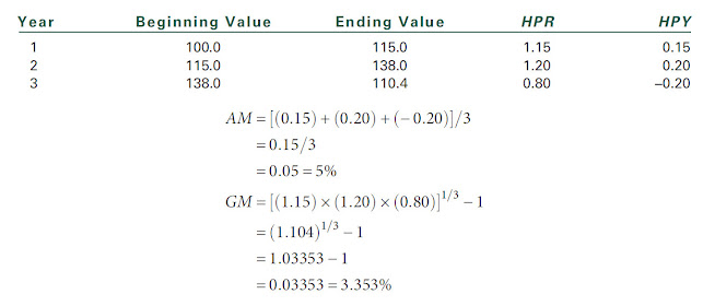
Single Investment Given a set of annual rates of return (HPYs) for an individual investment, there are two summary measures of return performance. The first is the arithmetic mean return, the second is the geometric mean return. To find the arithmetic mean (AM), the sum (Σ) of annual HPYs is divided by the number of years (n) as follows:

Where:

ΣHPY = the sum of annual holding period yields

An alternative computation, the geometric mean (GM), is the nth root of the product of the HPRs for n years minus one.

Where:

π = the product of the annual holding period returns as follows:

To illustrate these alternatives, consider an investment with the following data:

Read More